01 Tutorial — K-means + PCA

Cluster the Iris dataset with k-means, then unfold it onto a 2-D PCA scatter.

Module DataMining · KMeans + PCA Dataset bezdekIris · 150 × 4 Clusters k = 3 Output PNG + CSV

A complete unsupervised-learning pass over the classic Bezdek Iris table — 150 specimens, four morphological measurements, three hidden species — driven by a short VBScript run on the sciBASIC# script engine. The script loads the table with the DataFrame resolver, partitions it into k = 3 clusters, projects the four-dimensional points onto the first two principal components, renders an 800 × 600 Nature-themed scatter, and exports the fully annotated table as CSV.

02 Pipeline

Five statements, end to end

Step 1

Load

DataFrameResolver.LoadDataSet reads the CSV table and maps columns D1–D4 into k-means feature models.

Step 2

Cluster

dataset.kmeans(expected:=3) partitions the 150 specimens; ClassId() recovers the cluster label vector.

Step 3

Reduce

PrincipalComponentAnalysis(maxPC:=2) + GetPCAScore() unfold the 4-D points onto the PC1 / PC2 plane.

Step 4

Plot

A ScatterPlot (800 × 600, PlotTheme.Nature) colors every sample by its cluster id.

Step 5

Export

plt.SavePng writes the 300-dpi figure; result.saveto streams the annotated table to CSV.

01 The Script

Full demo source

The complete script exactly as executed by the sciBASIC# script engine (vbs.exe) — nothing elided.

kmeans.vb · 34 linesDownload kmeans.vb

#include "Microsoft.VisualBasic.DataMining.Framework.dll"
#include "Microsoft.VisualBasic.Data.Framework.dll"
#include "Microsoft.VisualBasic.Data.DataPlot.dll"
#include "Microsoft.VisualBasic.Math.Statistics.ANOVA.dll"
#include "Microsoft.VisualBasic.Drawing.dll"

imports microsoft.visualbasic.data.framework.storageprovider
imports microsoft.visualbasic.datamining.kmeans
imports microsoft.visualbasic.datamining
imports microsoft.visualbasic.data.framework
imports Microsoft.VisualBasic.Math.Statistics.Hypothesis.ANOVA
imports microsoft.visualbasic.data.plots
imports microsoft.visualbasic.drawing

dim file = "G:\GCModeller\src\R-sharp\REnv\data\bezdekIris.csv"
dim k = 3

dim dataset = DataFrameResolver.LoadDataSet(file, cols := {"D1","D2","D3","D4"}).ToKMeansModels()
dim result = dataset.kmeans( expected := k).toarray()
dim pca = result.CommonDataSet.PrincipalComponentAnalysis(maxPC := 2).GetPCAScore()
dim class_id = result.ClassId().ToArray()

SkiaDriver.Register()

Using plt As New ScatterPlot(800, 600, PlotTheme.Nature())
    plt.Title = "PCA group of bezdek-Iris"
    plt.SubTitle = "PCA score scatter with 3 iris species colors"
    plt.XLabel = "PC1"
    plt.YLabel = "PC2"
    plt.Plot(DataSerials(x:=pca!PC1,y:=pca!PC2, class_id).tolist())
    plt.SavePng("Z:/bezdekIris-pca-groups.png", 300)
End Using

call result.saveto("Z:/bezdekIris-pca-groups.csv")

03 Results

PCA scatter & cluster table

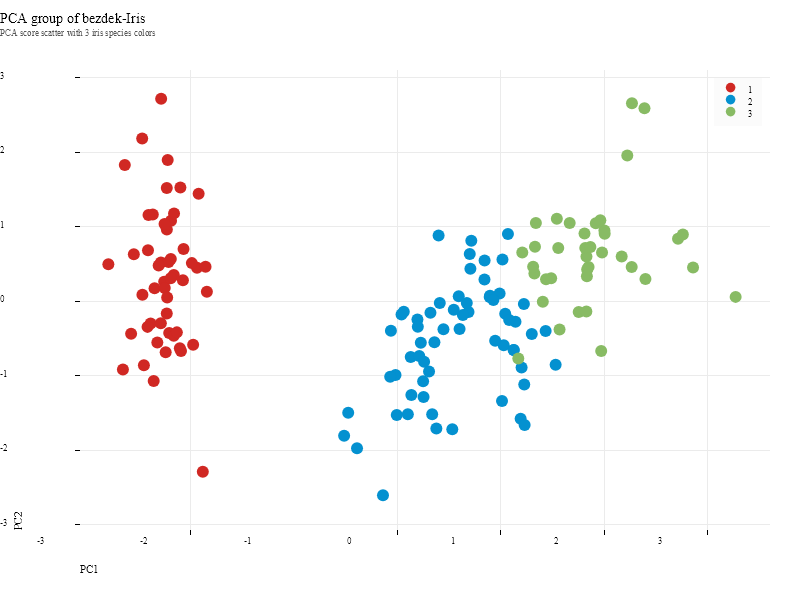
PCA score scatter of the bezdekIris dataset, 150 points colored by k-means cluster — **Fig. 1** — PC1 / PC2 score scatter of the Bezdek Iris table, 150 specimens colored by k-means cluster. Cluster 1 (red) — *I. setosa* — occupies a region of its own on the left; clusters 2 and 3 (blue / green) partition the morphologically intergrading *versicolor–virginica* range.

Table preview — `bezdekIris-pca-groups.csv`

The exported table keeps the original species label (ID) next to the assigned cluster number (class) and the four raw measurements. First rows, a middle slice and the last rows are shown; the full file holds all 150 data rows.

ID	class	D1	D2	D3	D4
Iris-setosa	1	5.1	3.5	1.4	0.2
Iris-setosa	1	4.9	3	1.4	0.2
Iris-setosa	1	4.7	3.2	1.3	0.2
Iris-setosa	1	4.6	3.1	1.5	0.2
Iris-setosa	1	5	3.6	1.4	0.2
···
Iris-versicolor	2	7	3.2	4.7	1.4
Iris-versicolor	2	6.4	3.2	4.5	1.5
Iris-versicolor	2	5.5	2.3	4	1.3
···
Iris-virginica	3	6.7	3	5.2	2.3
Iris-virginica	3	6.5	3	5.2	2
Iris-virginica	3	6.2	3.4	5.4	2.3

Species	Cluster 1	Cluster 2	Cluster 3
Iris-setosa	50	0	0
Iris-versicolor	0	48	2
Iris-virginica	0	14	36

K-means recovers I. setosa perfectly — all 50 specimens land in cluster 1 — and splits the overlapping versicolor / virginica pair 48–14 vs 2–36, the textbook result for this dataset.

kmeans.vb bezdekIris-pca-groups.csv bezdekIris-pca-groups.png