 sciBASIC#
↖
sciBASIC#
↖
03 Tutorial — Regression
Fit a line, cross-check a quadratic, and write the predictions back onto the table.
The regression convention in sciBASIC# is deliberately boring: X is the feature columns of a NumericTable, y is the label column you name. A synthetic dataset with deterministic sawtooth noise keeps the run reproducible — LinearFit lands on y = 2.0018x + 2.9862 with R² = 0.9988, PolyFit(2) confirms nothing better is hiding in the noise, and SetPrediction writes predictions and residuals back as new label columns for export.
02 Pipeline
From synthetic data to a fitted line
Synthesize
100 points of y = 2x + 3 + noise, where the noise is a deterministic sawtooth so every
run produces exactly the same fit. NumericTable.FromRows wraps it in the unified 2-D table
and table.SetLabel("y", y) attaches the observed values as the label column.
Fit
table.LinearFit(y := "y") returns a FitResult model carrying slope,
intercept, R², adjusted R², RMSE and residuals —
y = 2.0018x + 2.9862 with R² = 0.9988.
Cross-check
table.PolyFit(poly_n := 2) fits a quadratic for comparison: R² = 0.9988 — the
quadratic buys nothing, which is the point of a linear ground truth.
Write back
table.SetPrediction(model, withResidual := True) leaves the source table untouched and
returns a new table whose label matrix carries y, prediction and
residual columns.
Plot & export
A ScatterPlot (800 × 600, Nature theme) draws the 100 observed points plus a 50-point
model.GetY line series; result.WriteCsv exports the annotated table.
01 The Script
Full demo source
The complete script exactly as executed by the sciBASIC# script engine (vbs.exe) — nothing elided.
#include "Microsoft.VisualBasic.Data.Bootstrapping.Fittings.dll"
#include "Microsoft.VisualBasic.Data.Framework.dll"
#include "Microsoft.VisualBasic.Data.DataPlot.dll"
#include "Microsoft.VisualBasic.Drawing.dll"

imports Microsoft.VisualBasic.Data
imports Microsoft.VisualBasic.Data.Bootstrapping
imports Microsoft.VisualBasic.Data.Framework
imports microsoft.visualbasic.data.plots
imports microsoft.visualbasic.drawing

' ---------------------------------------------------------------------------
' Linear regression demo
'
'   dataset -> unified 2D table (NumericTable) -> LinearFit
'    -> prediction / residual written back to label columns
'    -> plot -> export csv
'
' The regression input convention is: X = all feature columns of the table,
' y = the label column named by the y parameter
' ---------------------------------------------------------------------------

' ---------------------------------------------------------------------------
' 1. Build a noisy linear dataset: y = 2x + 3 + noise
'
'    The noise is a deterministic sawtooth function so that every run produces
'    exactly the same fitting result
' ---------------------------------------------------------------------------
dim n = 100
dim features As Double()() = New Double(n - 1)() {}
dim y(n - 1) as double

for i = 0 to n - 1
    dim x = i * 0.1
    dim noise = ((i mod 7) - 3) * 0.1

    features(i) = New Double() {x}
    y(i) = 2.0 * x + 3.0 + noise
next

dim table = NumericTable.FromRows(Nothing, features, New String() {"x"})

call table.SetLabel("y", y)

call console.WriteLine($"dataset: {table.nsamples} samples x {table.nfeatures} feature")

' ---------------------------------------------------------------------------
' 2. Build the linear regression model
'
'    LinearFit returns a FitResult model object (slope/intercept/R2/RMSE/
'    residuals and so on are all carried on the model object)
' ---------------------------------------------------------------------------
dim model = table.LinearFit(y := "y")

call console.WriteLine($"linear fit  : y = {model.Slope} * x + {model.Intercept}")
call console.WriteLine($"R2 = {model.R_square}, adjust R2 = {model.AdjustR_square}, RMSE = {model.RMSE}")

' ---------------------------------------------------------------------------
' 3. Use a quadratic polynomial regression for comparison
' ---------------------------------------------------------------------------
dim quad = table.PolyFit(poly_n := 2)

call console.WriteLine($"poly fit(2) : R2 = {quad.R_square}, RMSE = {quad.RMSE}")

' ---------------------------------------------------------------------------
' 4. Write the prediction and the residual back into the label matrix of the table
'
'    SetPrediction does not modify the source table; it returns a new table with
'    the prediction columns written in
' ---------------------------------------------------------------------------
dim result = table.SetPrediction(model, withResidual := True)

call console.WriteLine($"prediction labels: {String.Join(", ", result.labelNames)}")
call console.WriteLine($"first row: y = {result.GetLabel("y")(0)}, prediction = {result.GetLabel("prediction")(0)}, residual = {result.GetLabel("residual")(0)}")

' ---------------------------------------------------------------------------
' 5. Draw the observed scatter points together with the fitted line
' ---------------------------------------------------------------------------
dim lineSize = 50
dim lineX(lineSize - 1) as double
dim lineY(lineSize - 1) as double
dim total = table.nsamples + lineSize
dim xs(total - 1) as double
dim ys(total - 1) as double
dim class_id(total - 1) as string

for i = 0 to lineSize - 1
    lineX(i) = i * 0.2
    lineY(i) = model.GetY(lineX(i))
next

for i = 0 to table.nsamples - 1
    xs(i) = table.Feature("x")(i)
    ys(i) = y(i)
    class_id(i) = "observed"
next

for i = 0 to lineSize - 1
    xs(table.nsamples + i) = lineX(i)
    ys(table.nsamples + i) = lineY(i)
    class_id(table.nsamples + i) = "fitted"
next

call SkiaDriver.Register()

Using plt As New ScatterPlot(800, 600, PlotTheme.Nature())
    plt.Title = "Linear regression of a synthetic dataset"
    plt.SubTitle = $"y = {model.Slope} * x + {model.Intercept}, R2 = {model.R_square}"
    plt.XLabel = "x"
    plt.YLabel = "y"
    plt.Plot(DataSerials(xs, ys, class_id).tolist())
    plt.SavePng(here("linear-regression.png"), 300)
End Using

' ---------------------------------------------------------------------------
' 6. Export the result table
'    (row names + x feature column + label:y / label:prediction / label:residual)
' ---------------------------------------------------------------------------
call result.WriteCsv(here("linear-regression.csv"))

call console.WriteLine("done: linear-regression.png")
call console.WriteLine("done: linear-regression.csv")
03 Results
The fitted line
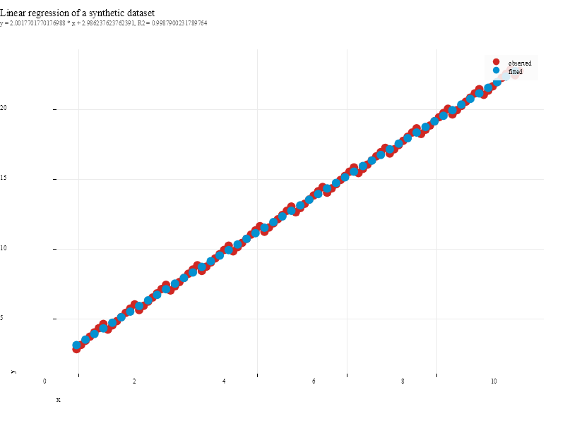
Table preview — linear-regression.csv
The exported table pairs the observed label:y with the model's
label:prediction and the signed label:residual for every sample. First rows and the
last rows are shown; the full file holds all 100 data rows.
| x | label:y | label:prediction | label:residual | |
|---|---|---|---|---|
| 1 | 0 | 2.7 | 2.986237623762391 | 0.2862376237623909 |
| 2 | 0.1 | 3 | 3.186414641464161 | 0.18641464146416098 |
| 3 | 0.2 | 3.3 | 3.386591659165931 | 0.08659165916593103 |
| 4 | 0.30000000000000004 | 3.6 | 3.5867686768677007 | -0.013231323132299355 |
| ··· | ||||
| 98 | 9.700000000000001 | 22.700000000000003 | 22.403408340834073 | -0.2965916591659301 |
| 99 | 9.8 | 22.3 | 22.60358535853584 | 0.303585358535841 |
| 100 | 9.9 | 22.6 | 22.80376237623761 | 0.2037623762376093 |
dataset: 100 samples x 1 feature
linear fit  : y = 2.0017701770176988 * x + 2.986237623762391
R2 = 0.9987900231789764, adjust R2 = 0.998777676476721, RMSE = 0.20111909379516651
poly fit(2) : R2 = 0.9987939843937537, RMSE = 0.20078961267610587
prediction labels: y, prediction, residual
first row: y = 2.7, prediction = 2.986237623762391, residual = 0.2862376237623909
done: linear-regression.png
done: linear-regression.csv
y = 2.7, predicted
2.9862376, residual 0.2862376. Because the noise is deterministic, the whole run
— and every digit on this page — reproduces exactly on your machine.